Products
Dynamic threshold estimation for anomaly detection

The quest for time-series anomaly detection at Sinch – part two
Many infrastructure and performance monitoring software tools offer built-in anomaly detection. But they often generate too many false positives. This is the second blog post in a series where we describe our journey in building a better performance monitoring tool for chatbots. You can find part one here.
Anomaly detection can also be formulated as a prediction problem. Anomalies are unexpected events, which makes them hard to predict. If you build a system that can predict the value of the next measurement quite well, you can compare that prediction with the actual measurement. If there is a large difference between what you predicted and what you measured, an anomaly probably occurred.
This blog post dives deeper into the methods we used to try and find out how big that difference should be before we consider it to be an anomaly.
Statistical threshold estimation
There are many machine learning methods out there to predict values for time-series. Some of them even come with tools to estimate confidence boundaries like ARIMA or Gaussian Processes. The output is typically a Gaussian, which tells you how likely it is that the actual measurement will fall between certain boundaries.
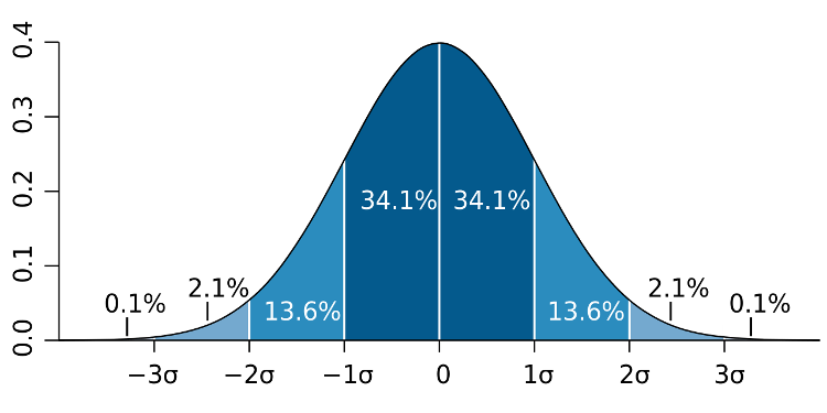
A commonly used approach is the 3 Sigma rule. If your measurement is more than three standard deviations away from your average, this measurement is considered an anomaly. But as illustrated in the image above, you still have a 0.1% probability that your prediction was incorrect; and that the measurement was, in fact, an expected value. Using this approach you actually build an outlier detection, but statistical outliers aren’t necessarily anomalies.
Imagine you have 100 corporate customers active in 100 countries. If you want to monitor their calls for each country every minute in real-time, you will have 10000 data points per minute for your anomaly detection algorithm to monitor. If you apply the 3 Sigma rule, you still have a 0.1% probability that your model might make an error. For this example, this means you will have 10 false positives per minute, or 36000 false alarms every day, on average, which is not the desired outcome.
You can, of course, change your confidence limit to 4 standard deviations and have only a little over 1000 false positives per day. But changing the accepted standard deviation is like setting your false-positive rate. It does not capture whether a measurement, in this case, a response time, is an anomaly or not.
Although the Gaussian distribution fits this expected output quite well in most cases, you could opt for a different probability distribution. But even if your new probability distribution fits the data better, you are fundamentally still using the same approach to the problem and setting the false positive rate of your anomaly detection model.
Anomaly score
There are methods like Robust Random Cut Forest (RRCF) that don’t work with Gaussian boundaries. RRCF is a tree-based method that tries to model the data. Every time a new data point is entered into the model, it checks where changes are needed to better fit the data. If the prediction was accurate, no changes are necessary, but if the prediction deviated a lot, the tree will need to be adapted to fit the model better.
RRCF returns an anomaly score that measures the change the model had to do to fit the data. If the tree in your model has a size of 256 (the default), the score can range anywhere between 0 and 256. Small changes in the model give you a low score, but if you have to change the entire tree, you can reach up to 256. If you want a range between 0 and 100%, you can simply divide the output by the size of the tree.
In general, you can set a threshold to, for example, a change of 50% of the tree. In our experiments, this worked quite well. However, we noticed that for some metrics, we still got too many false positives and quite a lot of missed events. With the moving average approach discussed in the previous blog post, we improved this, but the problem remained that we had to set a threshold for each metric to get the best performance. We noticed that picking the right tree size for each of the metrics was the issue. More stable metrics never used the entire tree, and more noisy data saw a lot of changes just to model the expected variance in the data.
Scaled minmax threshold estimation
To tackle the thresholding problem, we took a different approach. The idea is that you learn from past data what a good threshold looks like. Imagine you have a model that predicts your metric, the deviation from the actual metric can look like the graph below. If you want to apply this reasoning to the output of the anomaly score of RRCF, you can ignore the negative values in the examples that follow.
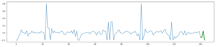
The blue line represents past deviations from the measurements. Green data points show the new deviations we’re trying to evaluate with our anomaly detection model. As you can see in the graph above, these green points are considered perfectly normal.
Over these six days, you can see there are two massive spikes in the blue line. If we assume that anomalies occur less than once per week, it’s a safe bet to assume that thresholds at the minimum and maximum of the past week work well, as illustrated in red below.
If we measure a new deviation from the predicted measurement of 0.75, we see that this approach doesn’t result in a detected anomaly. Using a statistical approach with three standard deviations will give you the purple line, as shown above, and a threshold at 0.4. That is not the desired behavior, and it explains why so many false positives are present when using this approach.
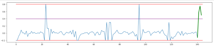
But this approach also has its limitations. Imagine you measure a deviation of 0.85. As illustrated in the graph below, this triggers the detection of an anomaly.
To avoid this, simply increase the boundary set. In practice, we noticed that increasing the boundary by 50% – or multiplying the boundary by 1.5 – gave us the best results. The reason for this is that only significantly larger deviations than past deviations trigger an anomaly.
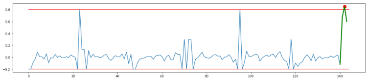
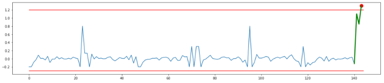
The example below illustrates the effect of applying a scaled threshold. A deviation from the predicted measurement of 1.3 triggers an anomaly, and deviations of everything below 1.2 don’t.
But if you have 3 data points, instead of just 1 that is significantly higher. You can apply the aggregation methods described in the previous blog post, such as the low pass moving average illustrated below (with a forgetting factor of 0.9).
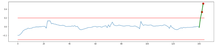
As you can see, this shows you can detect this anomaly after the second value even though this value was below the threshold in the previous example. That means combining the thresholding discussed here with the data aggregations method from the previous blog post allows you to catch more anomalies faster, without getting the false positives experienced with statistical methods.
In our experience, we got the best result by using the past eight days as history. That ensures you have each day of the week in your model and provides a bit more stability to allow for any holidays.
Since we typically use eight days of past data as history, it’s not possible to detect two anomalies in the same week. After an anomaly, it takes at least eight days before you can detect a similar anomaly. We are experimenting with methods to avoid this. The best solution we’ve found so far is to let our DevOps team acknowledge anomalies, so we can ignore them in our models. We are also experimenting with forgetting factors for these boundaries, but with no luck so far. We’ll let you know if we find something that works in another blog post.
Conclusions
In this blog post, we shared the approach we use to set thresholds for our anomaly detection model. For predictive anomaly detection methods, we use deviations from the prediction as an input signal. That ensures we can use time-series prediction methods to capture seasonality, but we don’t have to deal with the seasonality when determining the ideal boundaries. For methods that return a score like the RRCF method, use that as an input for this algorithm. We achieved our best results in practice by setting the detection thresholds to 1.5 times the maximum (and minimum) deviation measured.
Author: